Prior to 1983, the US Consumer Price Index included housing prices. A change was made at that time, however, to replace housing prices with a concept called “owners’ equivalent rent.” The rationale behind this change was that CPI should not include “investments” and home ownership was both consumption and investment. “Owners’ equivalent rent” was measured not by housing prices, but by rental prices given up by the homeowner in order to occupy the unit. In this way, it was hoped to strip out the “investment” related aspect of housing, while still holding onto the consumption aspect of it.
Unfortunately, this minor change in the way CPI was measured has had dramatic results on the end product. It’s created a situation where the Federal Reserve and other government actors are looking at one set of statistics to measure inflation, when the economic reality can be completely different. This is not to argue that there is a conspiracy to engineer the statistics, as some have suggested. Rather, a minor change in methodology has merely changed the way we perceive things in a detrimental fashion.
Alternative Economics
I’ve become enamored by how the disparity between official economic statistics and economic reality might have caused poor decision making by both the public sector and the private sector. As a result, I’ve launched a website, Alternative Economics, dedicated to exploring this issue in more detail. The centerpiece of my efforts is an Alternative CPI measure based on housing prices. From this, I’ve also re-examined GDP growth and monetary policy. The results have been paradigm-shifting, to say the least.
After viewing the economy under the lens of “Alternative CPI,” the US appears to have had negative real economic growth from 2000 to 2006. With high nominal GDP growth offset by even higher inflation, this period would be most properly termed “The Great Stagflation” or alternatively, “The Great Inflationary Depression.”
In this sense, 2000 – 2006 was the worst period in American economic history since the Great Depression and the ‘70s Stagflationary Era. While I’ve drawn several conclusions using my data, for now, I want to focus on my concept of Alternative CPI to show you why it’s more accurate and why it should change the way you think about the 2000s.
Alternative CPI Methodology
One major reason why housing price data is vital for any realistic inflation measure in the United States is because so much of American consumption is related to housing. Roughly 65% of Americans are homeowners and we have a society that views home ownership as an important goal in life. Mortgage payments often make up anywhere from 25% – 40% of monthly income for many Americans, making it a major cost.
Due to the effect of leverage in the housing market, it is one of the areas of consumer expenditure where prices are most likely to become inflated due to an excess supply of money. Given this, to ignore housing prices in inflationary measures is pure folly. Indeed, what’s the point of even examining CPI inflation if it ignores the most pertinent item in most American’s budgets?
For my conception of Alternative CPI, I’ve replaced the BLS’s concept of owners’ equivalent rent, with the S&P /Case-Shiller Home Price Index. This is slightly different than Floyd Norris’ conception in the NY Times, as he uses statistics compiled from Fannie Mae (FNMA.OB) and Freddie Mac (FMCC.OB). I decided to use Case-Shiller over this for a few reasons, including greater ease of access. Moreover, I would view it as an acceptable proxy for housing prices across the country.
In spite of the fact that urban housing prices would tend to rise more in a boom than rural prices, the majority of the American populace lives in a major metropolitan area. Urban housing prices would also be a better indicator of dangers in the real economy.
With Case-Shiller, there is both a 10-city index and a 20-city index. The 10-city index has a longer history, going back to 1987, while the 20-city index only reaches back to 2000. The obvious advantage with the 20-city index is that it looks at a broader swath of housing data. However, in practice, the two indexes do not dramatically differ from one another, as the chart below suggests - (click charts to enlarge):
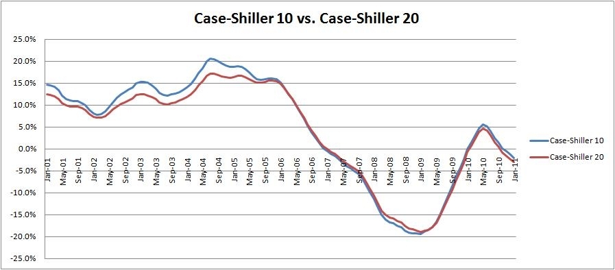
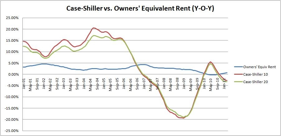
While the Case-Shiller 10-city index does show slightly higher year-over-year increases during the housing boom years, the differences are not that dramatic. In fact, if we take the above chart and add the BLS’s concept of “Owners’ Equivalent Rent” (OER), you will quickly see that the differences between the two Case-Shiller indices are minor compared with the difference between Case-Shiller housing price data and “Owners’ Equivalent Rent.”
Given this, I decided to use Case-Shiller’s 10-city housing price index in order to calculate Alternative CPI. The longer history associated with that index creates a better data set and it’s not a stretch to suggest that the Case-10 can serve as a proxy for a broader metropolitan housing market index.
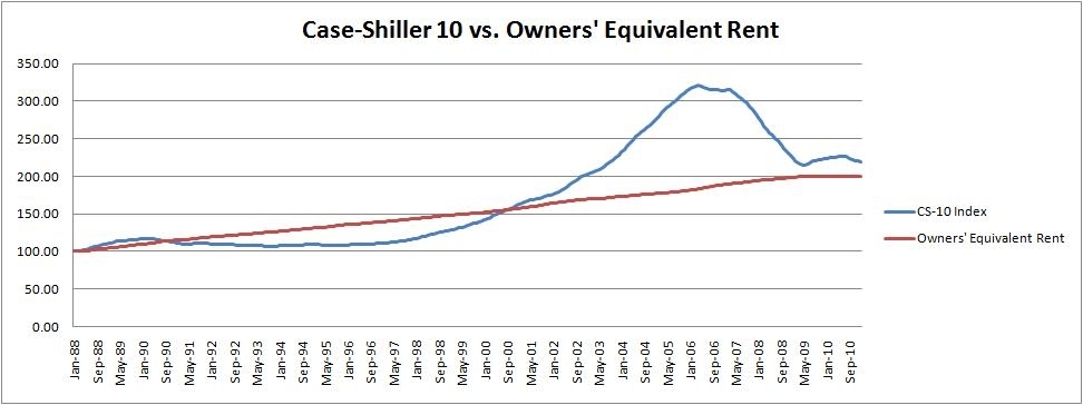
Before jumping to the results of our Alternative CPI, let’s take a look at one final chart examining the Case-Shiller Index versus owners’ equivalent rent. The chart below shows the index values, as opposed to year-over-year increases as in the chart above. The giant hill in the chart represents the housing bubble and you can see that we are just now reaching a point where the Case-Shiller 10-city index and OER are finally closing in on one another again:
Alternative CPI
Due to the failure of OER to capture true price inflation, it’s easy to see why Alternative CPI ends up being such an important concept. OER allowed official inflation figures to be dramatically understated for years and might have hidden major economic problems in the United States during the early 2000s. Moreover, it led to extremely poor policymaking from the Federal Reserve and the US government.
Let’s examine how Alternative CPI differs from official CPI. For my measure, I did not change any inputs in official CPI inflation except OER, which I replaced with the Case-Shiller 10-city housing price index. With this one minor change, CPI looks dramatically different as the chart below shows:

Official CPI and Alternative CPI stay within about a 200 basis point spread of one another from 1988 to 1998. After that, the two figures start to drift apart considerably. By 2004, there is nearly a 700 basis point spread between official CPI and our Alternative CPI measure.
In July ’04, for instance, official CPI records a mild 3.0% year-over-year increase in inflation. While this is lower than the Federal Reserve’s general target, it’s not all that alarming, all the same. 3% is well within US historical averages during healthy economic times.
Alternative CPI, on the other hand, reports a troubling 9.4% year-over-year increase in inflation. If official CPI had reported such a high result, alarm bells would’ve been set off all over the place. 3% is manageable inflation; 9.4% suggests an economy with major problems. In fact, we had already drifted over 6% inflation in 1999 using my Alternative CPI gauge. Alternative CPI cooled off a bit during the tech crash, before eclipsing 6% inflation once again by mid-2002.
Alternative Real GDP
Where this becomes even more profound is when we start looking at the Alternative CPI inflation compared with economic growth and monetary policy. I’m saving the monetary policy discussion for my next article, so for now, we’ll focus on economic growth. This is where our Alternative CPI starts to become “paradigm-shifting.” The chart below examines Alternative CPI versus Nominal GDP:
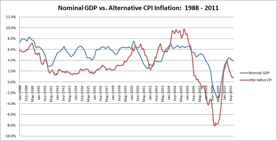
The best way to read the chart above is to examine both lines to see which one is on top. When the blue line is above the red line, that means that the US was experiencing positive real economic growth. When the blue line is below the red line, that means that price increases were outpacing nominal GDP growth, so that real economic growth was negative. Notice that the 2000 to 2006 period does not look all that terribly great under this prism.
Now, to make things a bit more clear, here is the data from the chart above reproduced into one Alternative Real GDP measure.
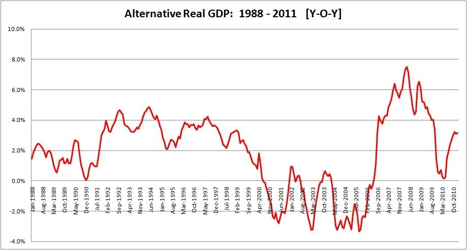
As you can see, from this perspective of the two charts above, the ‘90s was an era of great economic prosperity with positive growth almost the entire decade. Once we drift into the ‘00s, however, we have continued negative economic growth from 2000 till 2006. At that point, dramatic falls in housing prices lowered the real cost of living, thereby creating real economic gains.
In fact, surprisingly, according to this conceptualization, we’ve had more real economic growth from 2006 to 2011 than we did from 2000 to 2006. This isn’t because the US economy was doing exceptionally well in the latter period so much as the drop in real estate prices allowed for sustainable economic growth to resume; albeit, with a huge overhang from a weakened banking system holding things back a bit and stifling employment.
Hence, from this perspective of Alternative CPI inflation, the first half of the ‘00s appears as if it would be more aptly called “the Great Stagflation.” It should not be perceived as a period of prosperity, but rather, an inflationary depression, caused by poor monetary policy, misguided housing incentives, and an unneeded stimulus from the Federal government that only made things worse.
The Great Stagflation
Looking back, this period should have never been considered a “boom period” at all. Rather, it may have been the classic case of demand-pull inflation. In demand-pull inflation, unemployment actually falls below the “full employment” level, so laborers demand significantly higher wages. Unfortunately the small increases in productivity at this level (i.e. aggregate supply) are outpaced by increases in aggregate demand. This drives up end prices, resulting in inflation.
As such, the Great Stagflation should be examined as a more than just a boom; but actually, a depressionary boom, where an oversupply of money in the economy created a situation where the overall economy was experiencing negative returns on investment.
This was ignored largely at the time because Americans fell for two myths:
- Low unemployment signals a healthy economy
- Official CPI showed very low inflation, relative to economic growth
In my next article, we’ll examine monetary policy and how it helped contributed to the Great Stagflation. source